Tracking Production Downtime in Excel: Free Template & Instructions

Tracking Production Downtime to Improve Efficiency

Production downtime translates into an under utilization of capacity that impacts the bottom line. By tracking and analyzing production downtime, managers can identify production flow problems and develop action plans that focus on corrective and preventive measures. Identifying repeated causes for system and equipment malfunctions can lead to improvements in:

• Preventive maintenance programs
• Training and support for operators
• Quality control measures
• Equipment optimization standards

This example downtime tracking log can be downloaded here from Bright Hub’s media gallery and customized to work with different manufacturing processes. With further modification, the spreadsheet can also be adapted to track any “downtime” that may be causing delays in a project’s schedule.

What Production Data Needs To Be Tracked?

In setting up the spreadsheet, you will need to track production data to help you document the 5 Ws (who, what, where, when and why) to have a complete picture of what happened when the equipment came offline.

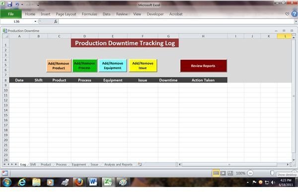
To begin, setup your data columns on Worksheet1 (renamed Log) to collect the following information related to the each downtime event:

• Date (particularly helpful for detecting issues that have implications for seasonal forecasting)
• Shift (by number)
• Product (name or code)
• Process (or work area involved)
• Equipment (name or code)
• Issue (reasons for the disruption)
• Downtime (documented in minutes, hours, etc.)
• Action taken (comments on the action taken, which can be used to develop a corrective action plan)

To make it easier to enter data into this Excel spreadsheet, create separate worksheets to store the lists that will be become drop down options on the log. Here are the ones used in the example spreadsheet to store lists and reports.

• Worksheet 2 – Shift
• Worksheet 3 – Product
• Worksheet 4 – Process
• Worksheet 5 – Equipment
• Worksheet 5 – Issues
• Worksheet 6 – Analysis and Reports (For example, charts to display downtime by shift, machine, process, and issue over time)

Steps for Creating Drop Down Lists

Once you have entered the items in each list on the appropriate worksheet, you can create drop down lists on the Log worksheet by following these steps:

• Highlight the cells on the Log Worksheet that you want to access a list. For example, for shifts, select B9 through B1000.

• Click on the Data tab.

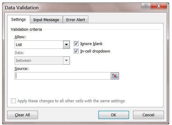
• Click on the Data Validation in the menu to bring up the dialog box.

• Click on the Settings tab in the dialog box.

• From the Allow menu choose List.**

  

  **

• Click on the Source line in the dialog box.

• Go to the worksheet with the list and highlight all the choices in the list plus blank rows for possible additions in the future. (Don’t worry the drop down list will not show the blanks.)

• Click OK in the dialog box.

A down arrow should appear in the cells on the Log Sheet to access the list.

Steps for Creating Command Buttons

To maneuver more easily between worksheets, you can create a set of command buttons to run a macro that will take you back and forth to the lists on the different worksheets. This will be helpful when adding and removing items in the list, such as when new equipment is brought on line or a machine is retired. A command button is a shortcut in Excel and is accessed through the Developer tab. Unfortunately Office 2010 does not display the Developer tab by default, so you will need to enable it using the following procedure:

To enable the Developer tab

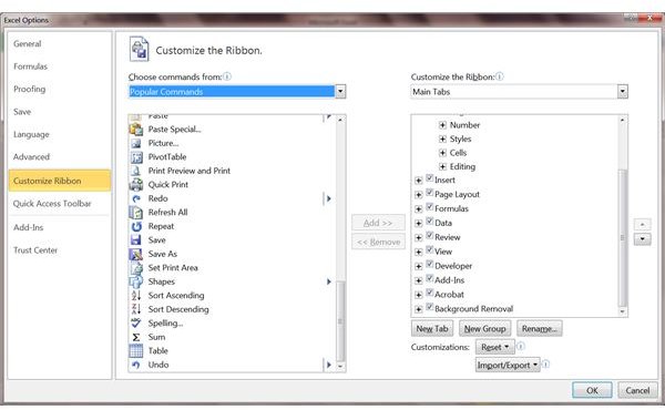
• On the File tab, choose Options to open the Excel Options dialog box.

• Click Customize Ribbon on the left side of the dialog box.

• Under Choose commands from on the left side of the dialog box, select Popular Commands.

• Under Customize the Ribbon on the right side of the dialog box, select Main tabs, and then select the Developer check box.

• Click OK.

  

You will now see the Developer tab on your ribbon, which will enable you to create command buttons.

To create and format a Command Button

• Select the Developer tab.

• Click on Design Mode and a dialog box will appear.

• Choose the Command Button (Active X Control) and then click the cell in which you want the button. You can adjust the size of the button just like a text box by stretching it out or pulling it in.

• To edit the button label, right click on the button and select the Command Button Object and Edit to change the button’s name.

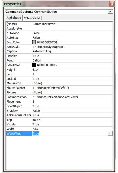
• To wrap the text on the button go to Properties on the Developer tab and this dialog box will open.

  

• Change WordWrap from False to True.

• To change the button color select BackColor then Button Face and then Palette.

To create a macro for the Command Button

• Right click on the Command Button.
• Select View Code and the framework for the macro script appears.
• Type in Sheet__.Select. For example to go to the Product worksheet type in “Sheet3.Select” into the macro or to return to the Log sheet from the Product sheet, type in “Sheet1.Select”.

Once you have a made all the changes, click on Design Mode again to lock and activate the button.

Generating Reports to Analyze Production Downtime

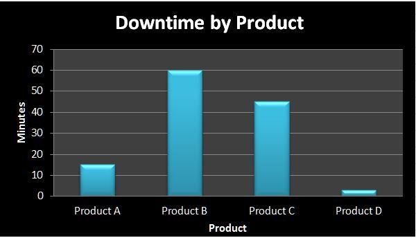
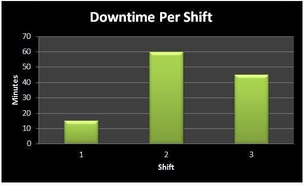
With the data in place, you can create various reports in the form of charts to analyze downtime by shift, product, process, equipment or issue. The Excel template includes two column charts that report total downtime minutes by shift and product.

To setup cells to show total downtime by product

Go to the Product worksheet and type in the cell next to the first product (Product A) the formula “=SUMIF(Log!C1:C1000,“Product A”,Log!G1:G1000),” which will add up all the downtime minutes affecting Product A from the Log.

Copy the formula to the other products and change “Product A” to the name of the other products.

To create a column chart to display total downtime by product

• Highlight the cells totaling the downtime from the Product Worksheet.
• Select the Insert tab and then Column Chart 2D.
• Click on Move Chart and in the dialog box that appears click on the drop down list under Object in and choose the Analysis and Reports Worksheet.
• Choose the Quick Layout on the Ribbon to select a pre-formatted chart or create one on you own. The one used in the template includes a title and axis labels with the legend removed manually.
• Repeat the process to create other reports that will update automatically to track downtime by shift, process, equipment, and issue.

For creating other types of charts, including a Pareto chart for root cause analysis, continue to this summary of Excel project management templates and tutorials available for downloading from Bright Hub.

References

Excel Help and How-to, Microsoft Office.com (accessed June 19, 2011).

“Poll: Common Causes Of Downtime In Your Data Center.” nixCraft, (accessed June 19, 2011).

Template design and screenshots created by author