This article describes the reason for the 1.5 Sigma Shift in simple layman’s terms without getting into detailed mathematics. It is an important concept in project management statistics which every manager needs to understand and appreciate in order to be successful in Six Sigma Projects.
What is a Six Sigma Process and where does the 1.5 Sigma Shift occur?
A popularly accepted definition of a six sigma process is one in which there are about 3.4 defects per million opportunities. i.e. Defects per million and the sigma level of a project can be used as project management statistics to evaluate the quality of a project.
The ideal goal for process capability is 3.4 defects per million which is almost negligible in number and considered a near-zero defect process. But, statistically a six sigma process means 2 defects per billion opportunities.
So, how did 2 per billion become 3.4 per million for a six sigma process? This is normally attributed to the 1.5 sigma shift
A layman’s perspective on the 1.5 Sigma Shift
To understand the math behind the 1.5 sigma shift in project management statistics, consider a desired goal which has to be achieved within a particular environment and certain environmental conditions.
- Any goal or result will have to be planned keeping 2 things in mind:
a. The goal itself under standard environmental conditions
b. Changing environmental conditions which may result in variation
However stable any process is, over an extended period of time, the environmental conditions change, which causes variation. Thus at the planning stage, these environmental changes need to be balanced by a compensation factor in order to account for these changes to ensure that the long term goal is met.
When expressed in an equation format, the following is obtained
“Short Term Goal = Long Term Goal + Appropriate Compensation Factor for Environmental Changes”
What is the 1.5 Sigma Shift? How is it applied?
Keeping the above equation in mind, consider the following
- In terms of project management statistics, 2 defects per billion opportunities in a project correspond to six sigma and 3.4 defects per million opportunities corresponds to 4.5 sigma.
- The overall goal is a near-zero defect process, or a 4.5 Sigma Level for the process in the long term.
- The environmental changes and the magnitude of this change is 1.5 Sigma (Calculated empirically by Motorola as the Long Term Dynamic Mean Variation)
Thus the Short Term Sigma Level (6) = Long Term Sigma Level (4.5) + Compensation Factor (1.5 Sigma Shift)
i.e. a Short Term goal of a 6 Sigma Level translates to 3.4 defects per million opportunities (4.5 Sigma Level) over the Long Term.
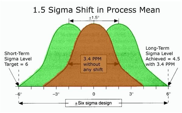
This is illustrated in the figure below.
The red area indicates the process without any shift in the mean.
The green area indicates the shift of 1.5 in the process mean.
Thus the short term sigma level aimed at is 6, in order to achieve a 3.4 PPM process corresponding to a 4.5 sigma level over a long term.
The objective in every project is to apply the DMAIC Methodology and bring the process sigma level as close to the goal of Six Sixma as possible.
For further information, view these articles on Six Sigma .