How is the Taguchi Method used in Six Sigma projects? We’ll take a look at some of the basic concepts and use an example to help illustrate.
The Taguchi concepts or Taguchi method talks mainly about the following three important statistical tools:
- Taguchi loss function
- Offline quality control
- Modified design of experiment using orthogonal arrays
This article will discuss only the simplified approach of design of experiment (DOE) and orthogonal arrays with a practical example.
-
DOE, which is used in Six Sigma , is a tool for selecting the set of parameters on which the experiment is performed. For example, if you want to do an experiment on heating of wire by passing the electricity through it, then you will have different control parameters like: wire material, wire diameter, wire length and these control parameters will have various values or levels. DOE will help you with selecting the parameters and their values most effectively and economically.
-
Taguchi’s DOE method makes use of orthogonal arrays, which drastically reduce the number of experiments to be performed, thus reducing the cost of the experiment.
Advertisement -
The orthogonal arrays (OA) are the predefined matrices of control parameters and number of experiments. The selection of the orthogonal arrays has to be based on the number of control parameters and their levels.
-
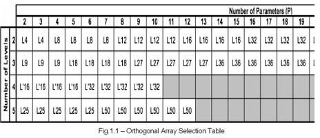
Various arrays as per Taguchi method are: L4, L8, L9, L12, L16 up to L50. The more numbers of control parameters, the higher the numbers after “L”. The following table will help you select what is suitable for your experiment:
-
For example, the wire heating experiment discussed above have three control parameters and two levels for each of the parameters, so, we have to select the “L4” orthogonal array from the table (Fig.1.1).
-
The construction of each OA is different. The construction of the “L4” OA is as below:
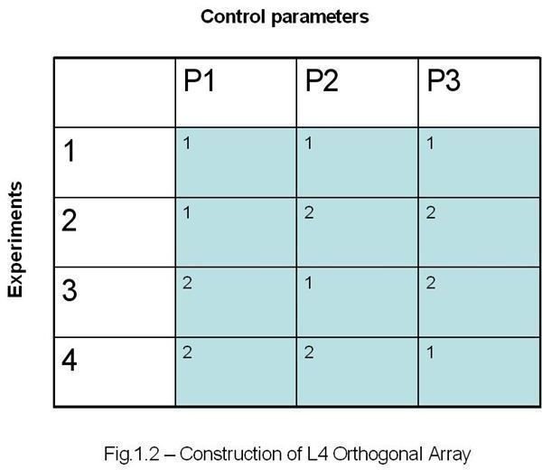
Where,
1 – First value of a parameter
**2 –**Second value of the parameter
- Once the OA is selected, then the trials (iterations) of experiments can be carried out. The number of trials are finalized based on the cost of performing the experiments and the complexity of the experiments. For the wire heating experiment discussed above may have three trials and at the end, we will have three result values for each of the four experiments.
- Next, the SN ratio for each of the experiments are calculated using the following formula:
SN = 10 log [(Sm – Ve)/ (N*Ve)]………………..eqn.1.1
Sm = (T1+T2+…..+Tn)2/N………………………eqn.1.2
Ve = Se/ (N-1)…………………………………..eqn.1.3
Se = St – Sm…………………………………….eqn.1.4
St = T12 + T22 +…..+Tn2…………………………eqn.1.5
Where,
T1, T2…Tn are the experimental results for the 1st, 2nd….nth trials respectively.
N is the number of trials.
- Next, the average values of the SN ratio for each level of each of the parameter are calculated and differences of the maximum and minimum values are tabulated. The highest of these values will have the greatest impact on the experiment. An example will help you get the idea clearer.
Practical Example
- Say, we want to use the Taguchi’s DOE method for finding the heat generated in a wire while passing electricity through it.
- Further assume that, you have only three control parameters namely wire material (P1), wire diameter (P2) and wire length (P3).
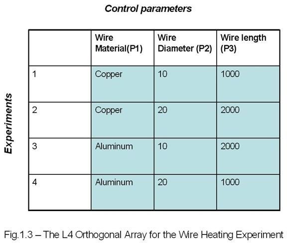
- Also, assume that all the control parameters have only two possible levels. Like, say, the wire material (P1) has two levels: copper and aluminum, the wire diameter (P2) has two levels: 10 mm and 20 mm, and the wire length (P3) has two levels: 1000 mm and 2000 mm. One of the levels will be represented as “1” and another will be represented as “2” throughout this DOE example. The next few steps will give you a clearer picture.
- Now, based on the number of control parameters and levels we have to select the suitable orthogonal array (refer fig. 1.1) and for our case the number of parameter are 3 and the number of levels are 2. So, we have to go for the “L4” OA. The Fig.1.2 above will give you an idea how the “L4” OA looks.
- Now, let’s put all the values to the L4 OA and it will become:
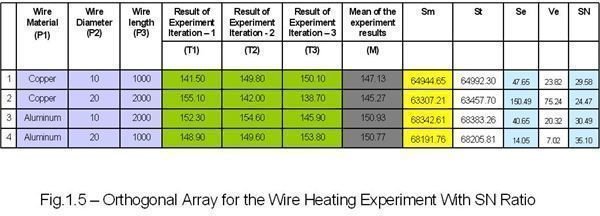
- Now, we have to perform the experiments and we will do three iterations of the experiment, the results are tabulated as below:
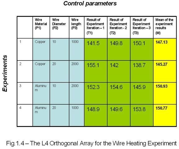
- Next, we have to calculate SN Ratio using the eqn.1.1, eqn.1.2, eqn.1.3, eqn.1.4 and eqn.1.5 explained above. I am showing the full calculation for one experiment below:
Sm1 = (141.50 + 149.80+150.10)2/3 = 64944.65
St1 = 141.502+149.802+150.102 = 64992.30
Se1 = St1 – Sm1 = 47.65
Ve1= Se1/ (N – 1) =23.82
SN= 10 log [(Sm1 – Ve1)/(Ve1*N)] = 29.58
The Rest of the values are tabulated below:
- Next, the average SN value for each parameter based on the levels is calculated. The calculation for the “Wire diameter (P1)” is shown below:
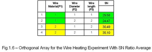
SNp11 = (29.58+24.47)/2 = 27.02 (average of the green cells)
SNp12 = (30.49+35.10)/2 = 32.79 (average of the yellow cells)
Difference (D) = 32.79-27.02 = 5.77
The rest of the data are tabulated below:
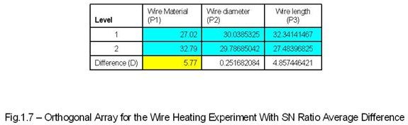
The difference (D) value decides the effect of the control parameter to the experiment. In our case the parameter “Wire diameter (P1)” has the maximum “D” value so it will have the greatest impact on the experiment.
Conclusion
The example of the simplified approach of the design of experiment (DOE) and orthogonal array discussed here is enough to understand the Taguchi concept of DOE. You can utilize this outline for complex Taguchi method DOE and OA as well. I think.
References
- https://controls.engin.umich.edu/wiki/index.php/Design _of_experiments_via_taguchi_methods:_orthogonal_arrays
- https://www.ee.iitb.ac.in/~apte/CV _PRA_TAGUCHI_INTRO.htm
Screenshots
- Figure 1.1 - https://controls.engin.umich.edu/wiki/index.php/Design _of_experiments_via_taguchi_methods:_orthogonal_arrays
- Figures 1.2 through 1.7 taken by Suvo