One of the best ways to learn how to compute a rolling average is to see visual working examples of the technique being used to solve a problem. After explaining the basic technique, we work through examples of using rolling averages to develop manufacturing and sales forecasts.
Moving Average or Rolling Average?
The averaging technique used in business practices titled “rolling average” can also be referred to as a “moving average.” These averaging techniques are calculated exactly the same way. The proper title to use for this averaging technique really comes down to how one prefers to visualize this technique in action; either rolling or simply moving.
How to Compute a Rolling Average
To follow along with how to compute a rolling average, please download The Basic Rolling Average Forecast Example , as it will be used to explain the calculations in this section.
The first decision a company has to make when calculating a rolling average is how many periods will be averaged; known as “n.” In the example, n = 4 periods. That is, four periods of historical data will be used to develop the rolling average. A company must choose the number of periods they want to average based on how reactive they want the rolling average to be with recorded data changes. The more periods averaged, the less reactive the rolling averages will be; which means using only a few periods, such as one or two, will provide very reactive rolling averages—but then, with that little data, you might as well just use a standard average.
Computing a rolling average requires data recorded over several consistent time periods. Usually, historical data, such as historical sales, production, or even profits made; is used. This rolling average produces a future value, known as a forecast. A forecast is a calculated prediction of any type of future data for the next business period; including daily, weekly, or monthly forecasts; based on the most recent number of periods, “n,” of historically recorded data being used in the calculation.
More specifically, a rolling average can be defined as a continuously moving, calculated average of the most recent number of periods; “n,” defined by the company. Let’s take a look at the example to see how this calculation works.
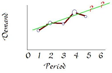
In Table 1 of the example, the first forecast calculated is for period five; which is 775. This was calculated by averaging the four most recent historical pieces of data right before period five indicated with red check marks, since “n = 4 periods” for this example. The detailed calculations for period five’s forecast are explained in Table 2. Once the actual data for period five is collected and recorded into the table, the forecast for period six can be calculated.
The rolling average forecast for period six is calculated based on the four most recent historical pieces of data before the sixth period; an average of the historical data for periods two through five, indicated with blue check marks. The forecast is then documented in the table, which is the blue “825” forecast for period six in Table 1 in the example. In order to see the detailed calculations for the sixth period’s forecast, please see the second row of Table 2 in the example.
To find out how to compute a rolling average forecast using two variables, please continue reading on Page 2.
Using a Rolling Average with Multiple Variables
Once one understands how to compute rolling average calculations with one variable to find a single forecast, such as sales or number of units sold; the next step is learning how to compute more advanced statistics with the rolling average technique by using two variables.
In order to follow along with the rest of this section, please download the Advanced Rolling Average Example ; which is a Microsoft Excel file contains an example of using the rolling average method with two sets of variables.
In this example, two sets of historical data are presented, which are the total amount of sales in dollars listed in column B and the number of sales in column C. By using these two sets of data, an average amount of money earned per sale can be calculated; as seen in column F. Let’s take a look at how to perform the calculations.
First, take a look at the equation to calculate a rolling average using two variables. Notice that each variable must be added up before the division between the two variables occur. Never compute an average of each period separately and then average the results, as this will provide an incorrect forecast.
The first forecast in the example is for period 5. To compute the rolling average for period 5, the first four pieces of “Sales $” data from column B must be added up; since “n=4 periods” in this example. Then, the first four pieces of “Sales #” data from column C must be added up. Finally, the total from the first four periods of column B must be divided by the total calculated from column C resulting in a calculated rolling average sale that will be encountered in period 5. In order to see a detailed explanation of the exact calculation used to find the forecast for period 5, please refer to Table 2.
Once period 5 is expended, the average can move down to calculate the rolling average sale for period 6, based on the four most recent pieces of data in each of the historical data columns. The process then continues for every period.
The Difference Between Standard Average & Rolling Average
In order to visually see the difference between standard average and rolling average calculations, please download The Standard Average vs. Rolling Average Example ; a Microsoft Excel file explaining the difference between a working standard average example and rolling average example.
As seen in the example, a rolling average forecast is calculated with a simple standard average. The first calculated average for every company is a simple standard average calculation. However, every forecast after the first standard average forecast is considered a rolling average forecast.
A rolling average calculation has one concept very different from a simple standard average calculation. First, a standard average is calculated by taking a set number of pieces of data, adding them together, and dividing the total by the number of pieces of data used, referred to as “n.”
Yes, this is a part of the rolling average technique; however, the main concept of a rolling average forecast is how the standard average continuously “rolls” to the next set of most recent number of periods, “n.” The process of continuously moving the average to the next set of most recent set of “n” periods is the one differentiating a standard average from a rolling average forecast.
Please continue onto Page 3 in order to learn how to compute rolling average manufacturing and sales forecasts.
Computing Rolling Average Manufacturing Forecasts
The manufacturing forecast can calculate how many items to produce to meet the demand of the company’s buyers, known as production planning; or to calculate how many items to stock on in a store, known as demand planning. In order to follow along with how to compute rolling average manufacturing forecasts, download Computing Rolling Average Manufacturing Forecasts ; a Microsoft Excel file containing two working examples of a rolling average manufacturing forecast calculations.
The Production Planning Forecast - (Page 1)
Production planning in a manufacturing facility depends on the amount of units forecasted to be demanded by buyers in the future period. As seen on Page 1, to compute a rolling average “Production Planning Forecast” to predict how many units to manufacture a company must know how many units were demanded in the past “n” number of periods. The recent number of “n” periods are averaged in order to create a forecast. As one more month is complete, the number of “n” periods averaged “rolls” to average the latest “n” periods. This can be seen in the example.
The number of periods used is four periods, as stated by “n=4 periods.” Period five is forecasted by averaging periods one through four; period six is forecasted by averaging periods two through five; and so on.
If more periods are used to compute a rolling average forecast, the forecast will be less responsive. Using only two to four periods is usually the normal number of periods manufacturing companies use to compute production planning forecasts.
The Demand Planning Forecast - (Page 2)
After closely analyzing Page 1, the “Demand Planning Forecast” example on Page 2 may strike a very close resemblance. The examples on both pages are practically the same; however, in demand planning historical data of the number of units sold to buyers or customers will be the best metric to compute a rolling average demand planning forecast more accurately.
How to Calculate Moving Average Sales Forecasts
A moving average sales forecast is calculated the same way as a manufacturing forecast. In order to see a moving average sales forecast, download the Example of a Moving Average Sales Forecast . This is also an Excel file, like the Computing Rolling Average Manufacturing Forecasts featured in the previous section; however, this file has three pages. The extra two pages contain examples of “Weighted Moving Average Sales Forecasts” and “Exponential Smoothing Sales Forecast.”
For more details on all three forecasting examples featured in the Example of a Moving Average Sales Forecast, please check out the Complete Working Example of a Sales Forecast for 3 Forecasting Methods .
Sources
Information:
Berry, W. L.; Jacobs, F. R.; Vollmann, T. E.; Whybark, D. Clark. Manufacturing Planning and Control for Supply Chain Management.
(2005). Chapter 2: Demand Management (p. 17-52)
Images: Created by the author of this article, Christopher Kochan.
Media Files: All the media files featured in this article were created by the author, Christopher Kochan; specifically for the readers of this article.
This post is part of the series: Averaging Techniques: Manufacturing and Sales Forecasting
This series features averaging techniques used by project managers to calculate manufacturing forecasts and sales forecasts.