Illustrating the Rolling Forecast Method for Time and Expense Management

What’s Wrong with the Conventional Budgeting Method?

Given the volatility of current business conditions, making financial projections based on past project costs is like working under a “bad cloud” – the projected financial plan doesn’t hold much water anymore. In fact, the elements that could cause variations between the estimated and the actual costs are many; thus, most project managers tend to be slow in making adaptive decisions.

This dilemma gives justification to the current trend of shortening the projection or budget period, as it allows a company to work with a more realistic set of financial views. The method being employed is the rolling forecast (RF) system, in which the objective is not to look too far behind or way ahead but, instead, on what is up to date. Finding out the causes of variations becomes a task much easier to handle; hence, adjustment processes and making new business decisions goes faster.

Cost-savvy project managers get into the groove by applying the same technique in managing the time and costs they allot to their undertakings. Get insights on how the method is applied, as this article proceeds with a discussion of its mechanics.

Explaining the RF Technique

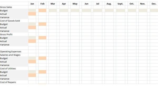
Visualize an RF budget for a twelve-month period by clicking on the first image provided.

The green cells represent the initial projections for the 12 months. At the end of a specific timeframe, which in our example is on a per month basis, the data for the actual costs are entered and the variances, extracted. Take note that the inputs for actual costs are assigned with a brown color code, which serves as a guide.

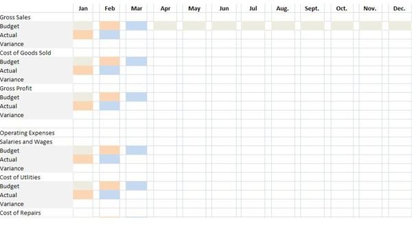
After the first month’s budget has been analyzed, the RF method proceeds by adjusting the succeeding month’s budget using the actual costs incurred during the previous month.

Notice on the second image that the cells for the February budget are now brown instead of green, which means that the actual costs incurred in January were keyed-in as the forecasted amounts for February.

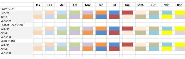
The same procedure will be adopted throughout the 12-month period. Take a closer look at the other image and study the color pattern, as each new color code is rolled-over to the following month.

Comprehend the objectives of keeping forecasts up to date as we provide an example of how this can be used for time and expense management of projects.

Using the RF Technique for Time and Cost Monitoring

In as much as planned project costs are determined for each stage or phase of work, the budget projections in our example are set under similar conditions.

However, our presentation is different since figures are analyzed on a per week, per hour and per cost basis.

The progression of the color pattern is on a downward trend as our objective is to monitor the remaining budget allocations for a particular stage of work.

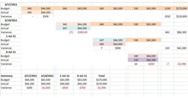
Our budget example is for Stage 1 with a total projected cost of $175,000 to be accomplished at an allotted time of 1350 hours. Time and costs are spread out within a 4-week period and are presented in their original amounts in the first week.

Week 1

Actual costs incurred for the week ending June 17, 2011 were $44,200 resulting in a positive variance of $300. We can easily surmise that the savings was achieved from other expenses not related to salaries, since there was no variance between the budgeted and the actual number of hours.

The budget allocation of $43,500 for the second week is lower than the actual expenditures of $44,200 of the first week. Still, it is deemed that the latter amount is more realistic than what was initially projected. Hence, the budget was adjusted for the week ending June 24, 2011 by using the latter amount.

Week 2

Review of the total projections for the week ending June 24, 2011 disclosed variances for both time and costs. This denotes that the savings of $300 was not maintained because the total number of hours spent (347 hours) was more than the 340 hours allotted. Keep in mind however, that the primary objective is to keep project activities in pace with present conditions, and not the attainment of cost savings.

The project manager can easily investigate as to whom among the team members spent more time in performing the task that was assigned. Was there additional work performed? Were there errors and recalculations made? Or were the concerned members merely slacking off?

Taking up this issue during the weekly meeting will make team members aware of how closely you are monitoring the time schedule. In fact, best practices recommend that for a budget or forecast to be effective, its significance and the rationality of its purpose should be discussed among the direct participants.

In this particular scenario, you can elaborate on how the $300 savings you achieved was voided by the additional hours spent. If the team was working under the same conditions, it would have been possible to maintain the week’s expenditure at the budgeted amount.

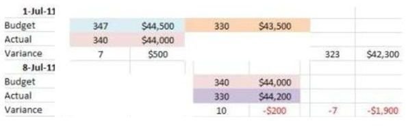
Week 3

The actual costs and hours of week 2 were rolled over as the budget for the third week of Stage 1, while the latest results of the time and cost monitoring ended on a positive note. Obviously, the timeframe was met and, perhaps, a conscious effort to avoid additional costs produced the desirable results.

Week 4

On the final week, it appears that work went on smoothly since tasks were accomplished according to the original number of hours estimated, which is 330. The cost allocation, however, was short by $200 despite being adjused to real time costs. It appears that the prices of the additional costs incurred have increased, or some unforeseen purchase may have surfaced. There’s also the possibility that it’s simply a matter of underestimation, since the original cost projections of $43,500, for the final week is lower than the rolled-over estimate of $44,000.

An overall assessment of the rolling forecast makes the user realize that had the projections stayed at the original estimations, the resulting variances would have been higher. (See the summary of hours and costs in the sample provided.) As project manager, such variances would have prompted you to run the operations at a less realistic condition.

A more comprehensive discussion on how to make forecast estimates can be gleaned in a separate article entitled Managing Cash Flow Control in Construction Projects. The budgeting method used however, is different since it makes use of the “contingency-principle” by adding a reasonable estimate of contingent outlay in anticipation of cost inflation. Considering the cost intensive nature of construction projects, the rolled-over expenses were further modified by adding additional amounts as buffer.

Summary

Although projections are basically developed from historical costs, keeping the gap nearer between past and present enables the decision makers to manage and take action at a faster pace. Explore the benefits of using the rolling forecast method for your budget projections during these times, in which uncertainty of business conditions often prevail.

Reference Materials and Image Credit Section:

Reference:

• Use a Rolling Forecast to Spot Trends – https://hbswk.hbs.edu/archive/5250.html#top

Image Credtis:

• GNU Free Documentation License, Version 1.2 / Wikimedia Commons
• Screenshot images of Rolling Forecast visual aid were created by the auithor for this article.