How is Little's Law Used in Lean Six Sigma?
Understanding Little’s Law
This law is termed Little’s Law because it was postulated by a former professor from the Massachusetts Institutes of Techology named John D. C. Little.
In its original form, the law can be explained using queuing theory as follows,
L = λ W
- ‘L’ denotes the long-term number of customers in the system.
- ‘λ’ denotes the long-term average arrival rate.
- ‘W’ denotes the long-term average time a customer spends in the system.
A more generalized version of Little’s Law is shown below:
No. of Units in the Process = Completion Time per Unit X Time in the System
Applications of Little’s Law
Little’s Law has a variety of applications and can be used in the following areas.
- Queuing
- Project Management
- Transactional Processes
- Lean Six Sigma
- Manufacturing Processes
A Simple Example
The applications of Little’s Law in Lean Six Sigma are illustrated below with a simple example.
A Lean journey usually attempts to reduce or eliminate waste in the system and improve speed, efficiency and overall effectiveness of the system. Minimizing waste includes an analysis of inventory on-hand and taking appropriate steps in order to reduce that inventory.
This can be done using the Little’s Law equation which addresses the relationship between Work In Progress (WIP) inventory, the Lead Time and the Average Completion Rate (ACR).
WIP = Lead Time X ACR
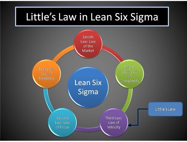
Little’s Law is also known as the Law of Velocity and is one of the Five Laws of Lean Six Sigma.
Assume that there is a small company, and from the historical data it is seen that the company’s average project completion rate is 5 projects every month, and each project takes an average of 8 months to complete.
Then the Little’s Law equation is given by:
40 Projects = 5 Projects Per Month X 8 Months Per Project
Now, if the company has used process improvement via Lean Six Sigma techniques in order to improve the completion rate, and the average completion rate increases to 6 projects per month, then the improvement in the lead time of completion can be visualized as follows.
-
New Lead Time = (40 Projects / 6 Projects Per Month) = 6.67 Months
-
Improvement in Lead Time of Completion = ((8-6.67)/8) *100 = 16.67% Improvement
Thus Little’s Law can be utilized to judge the impact of Lean Six Sigma.
Widespread Applications
The beauty of Little’s Law lies in its simplicity. The law also has widespread applications and can be utilized in everyday life, too. Any situation that involves waiting time can be studied using Little’s Law. Knowledge of any of the two constraints will help determine the third constraint. This is a very simple way to learn about the three factors that guide a system and how to effectively manage them.
The recommendation for project managers is to try and use Little’s Law in everyday life in order to better understand its implications. Doing so will also help them to visualize more applications of Little’s Law in their work life.