How to Create a Fishbone Diagram in Excel

Fishbone Diagram in Excel

Fishbone, or cause and effect, diagrams are often used in project planning sessions to identify all of the components, both man and machine, that go into any workflow process. Once these components are identified, it’s a lot easier to look at each one and see where problems or inefficiencies are creeping into the process. While there are some dedicated project management applications that will help in the construction of fishbone diagrams, you can also create these visual aids yourself. Here, we’ll show how to make a fishbone diagram in Excel.

How to Create a Fishbone Diagram - Step 1

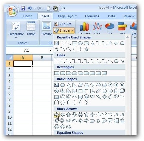
We’ll begin by constructing the main arrow in the middle of the fishbone diagram. Go to the Insert tab on the Excel ribbon and click on Shapes. Click on the first arrow in the Block Arrows category. Or, you can pick any of the other arrow shapes if you prefer. (Click any image for a larger view.)

[caption id="" align=“aligncenter” width=“600”]

Click anywhere in the spreadsheet and the arrow will be placed. Once the arrow has been placed, you can move and resize it to the location and shape you like. Here, we’ll make the arrow longer and place it in the middle of the visible spreadsheet area.

[caption id="" align=“aligncenter” width=“600”]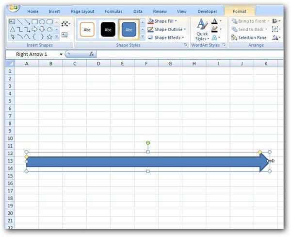 Move and Resize the Arrow[/caption]

If you don’t like the default choices of color and style, you can make changes to these on the Format tab, but for now, we’ll keep the default options.

Step 2

Now, we want to insert the lines that converge into the main arrow. Return to the Insert tab on the Excel ribbon and click on Shapes again. This time select the single-headed arrow (the second item) in the Lines category.

[caption id="" align=“aligncenter” width=“600”]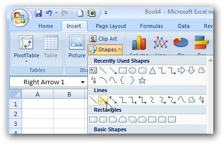 Insert Line Shape[/caption]

Click someplace on the spreadsheet to insert the line. Don’t worry too much about the position since we’re going to need to move it anyway after we resize it. Click and drag one of the endpoints of the line to resize and change the angle of the object. The screenshot below shows this action in process.

[caption id="" align=“aligncenter” width=“600”]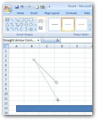 Process of Lengthening and Changing Angle of Line in Excel[/caption]

Next, drag the line to the desired position on the spreadsheet.

[caption id="" align=“aligncenter” width=“600”]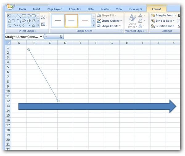 Place the Line in Desired Position[/caption]

If you want to make the line wider, right-click on the object and select Format Shape.

[caption id="" align=“aligncenter” width=“600”]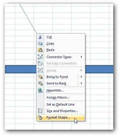 Format Shape[/caption]

In the Format Shape dialog box, make sure that Line Style is chosen from the list on the left and modify the value for Width.

[caption id="" align=“aligncenter” width=“600”]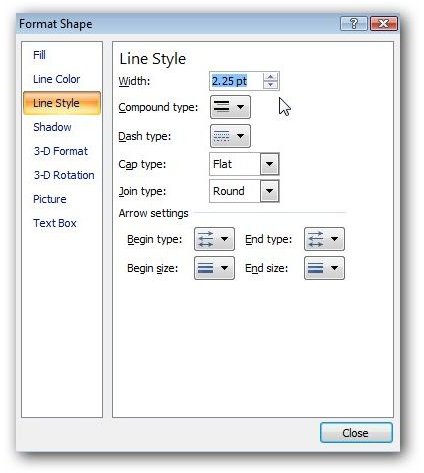 Change the Width of the Line[/caption]

Click the Close button when done to return to the Excel spreadsheet. Here’s what our diagram looks like so far.

[caption id="" align=“aligncenter” width=“600”]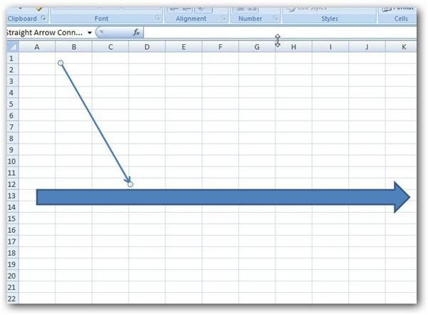 Diagram after Adding One Line[/caption]

Step 3

Now, we want to insert additional lines, but rather than perform Step 2 for each line we want to add, we’ll use a shortcut. Right-click on the existing line and select Copy. Then, right-click on any other area in the spreadsheet and select Paste. This will create a copy of the line create in Step 2 that can be moved to any other location on the spreadsheet. Do this for each additional line that you want to create. Note that you if you are placing lines above and below the main arrow of the fishbone diagram, then you may need to rotate the lines in the bottom portion. The most accurate way to do this is to right-click on the line and select Size and Properties.

[caption id="" align=“aligncenter” width=“600”]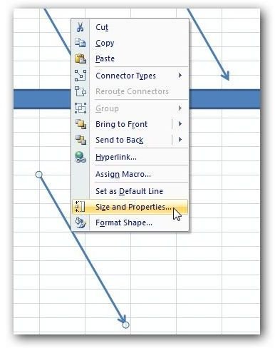 Select Size and Properties[/caption]

On the Size tab of the Size and Properties dialog box, adjust the rotation either by typing in an exact angle value or by clicking the up/down arrows until you find the angle you want. Here’s a sample of a fishbone diagram where the lines converging into the main arrow from above have a rotation of 270 degrees, and the ones below have a rotation of 150 degrees.

[caption id="" align=“aligncenter” width=“600”]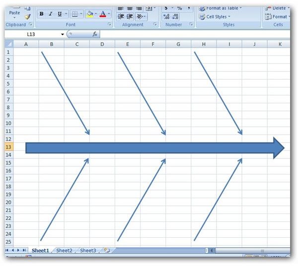 Diagram with Several Lines[/caption]

Step 4

The next things we need to add are text boxes. While you could try typing text directly into any of the cells surrounding the diagram, the end result probably won’t look very well formatted. Plus, if we use text boxes, the information can easily be moved around to different locations of the diagram, if needed, without having to move the rest of the diagram. To add a text box, return to the Insert tab on the Excel ribbon and click on Text Box. Click on the place in the spreadsheet where you want to insert the text box. Click and drag any of the corners of the text box to resize it to your desired size and shape. We didn’t worry too much about formatting any of the other objects yet, but it’s a good idea to apply some basic formatting to the text box so you’ll be able to see it easier on the diagram when it’s not selected. With the text box, still selected go to the Format tab under Drawing Tools on the Excel ribbon. From the Shape Styles category, select a formatting style for the text box.

[caption id="" align=“aligncenter” width=“600”]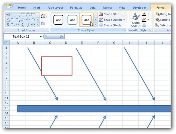 Choose a Style for the Text Box[/caption]

Step 5

Just as with the lines we added to the fishbone diagram, the easiest way to add more text boxes is to copy and paste the one created in Step 4. Then you can select each new text box and drag them to a new position on the spreadsheet in any manner you desire.

[caption id="" align=“aligncenter” width=“600”] Sample Fishbone Diagram Layout[/caption]

Additional Resources: If you’d rather start out with a pre-designed fishbone template that you can modify to fit the needs of your project, you can find one in this collection of Six Sigma templates. Similarly, if you’d like to learn how to use Excel to create other project management charts and diagrams or find additional free templates that you can download, check out this collection of Excel templates and how-to guides.